
Application
note
Differential cell count, ie counts of cells in different groups within a cell culture is a very common read-out in cell culture-based research. FACS is the de-facto standard method for determining differential cell count; it has certain drawbacks in terms of cost, applicability and robustness that can be addressed by image-based methods if image analysis can be made cheap, fast, and robust.
We present dot-placing as a method for image-based differential cell counting and use a publicly available dataset to demonstrate how it can be implemented quickly, easily, and without any image processing knowledge in our VAIDR system for integrated image acquisition, image analysis and data analysis
Introduction
One of the simplest and most common read-outs in cell culture based research is cell count. Depending on circumstances, it can be an indicator of cell health, cell identity, treatment toxicity, treatment effectiveness, and others. Methods for determining cell count are cheap and easy to come by.
Still simple and common, but slightly more difficult to determine is differential cell count, ie counts of cells in different groups within a cell culture. These are relevant eg where cells can change their identities, when the ratio of cells affected by some treatment is a relevant metric, or in co-cultures, where only one of the cell types present is the cell type of interest in an experiment. Fluorescence-activated cell sorting (FACS) is a well-established method to determine differential cell counts.

“The good thing about FACS is that it is well-established and well-understood. What's bad about it are the cost, the labor, and the variability.”
Dr. Thomas Frahm
Head of BD, Scientific Advisor at TRI
However, FACS has several drawbacks:
- FACS machines are expensive,
- their operation is labor-intensive,
- they must be calibrated for each application,
- cells must be detached,
- cells must be stained in a way that is specific to their group.
These drawbacks lead to high costs, limit the applicability of FACS, and introduce variability.
Image-based differential cell counting, on the other hand, has the benefit that imaging is often cheap, fast, and robust. Also, the same image data set can often be used for different purposes. Images can be analyzed and re-analyzed, cells can stay in place, and the sample can often stay undisturbed by the process.
The downside is that image analysis, in contrast to imaging, is not necessarily cheap, or fast, or robust. Without a good starting point, developing an imaging analysis method takes time and it requires a very specific and rare skill set that does not overlap much with those required for cell culture and cell Biology. Applying a method, once it is developed, depends on the fragile interplay of software and hardware components. For consistent results, usage of tools needs to be uniform, and the handling of primary and meta data must be meticulous.
Some common software tools for image analysis, including for differential cell counting, have been developed. Some are free and open source (FOSS), some are paid for. Considering the time and skills required to develop an image analysis method, even some of the most expensive commercial solutions can be worth their price if one is trying to solve the particular task on the particular kind of data for which they were developed.
If there is no ready-to-use method for a particular task, or if imaging (imaging modality, imaging parameters, staining), cell type, or culture conditions differ, one is on their own.
For image-based differential cell counting to be as cheap, fast, and robust as imaging alone, both the development and application of image analysis methods must be cheap, fast and robust. This means that development must not require:
- rare skills,
- inordinate amounts of manual labor,
- too much experimentation—it must ‘just work’ for most applications.
Application of an image analysis method must:
- not require the attention of an expert,
- be as automated as possible (avoiding delays, effort, and variability),
- be powerful enough to handle the full variability of the data generated by the biological processes.

“Scripting image analysis is fun—but it isn't sustainable. There's just not enough time and talent around to hand-craft a solution for every need. And that means that needs are unmet unless we automate.”
Johannes Bauer
CTO at TRI
Classical image analysis does not satisfy these criteria. While there are good, powerful, and often free products out there that support it, and great research is done with their help, using these products takes a good mathematical understanding of the problem at hand, a lot of trial and error for all but the simplest cases, and even then, considerable time. The results are usually not turnkey solutions but rather script files that perform the raw image analysis but leave the data logistics and the analysis of the results to the user.
In recent years, machine learning has become a popular approach. It promises results without having to worry about how to solve a task at the numerical image level. Image segmentation methods in particular are the family of machine learning methods most naturally suited for the task of counting objects: image segmentation is the task of segmenting an image into regions indicating the kinds of objects represented in those regions. The segmentation of an image into regions representing the background, cells of type A and cells of type B, is a good first step to counting cells of either type.
Unfortunately, image segmentation methods that are powerful enough to capture the subtle differences between different cell types are notoriously difficult to train and tune, both at the technical and methodological level and they require powerful hardware. Also, to train a segmentation algorithm, one needs to supply a sizable amount of pre-segmented image data, and segmenting enough data by hand can be tedious, even with good tool support.
We therefore introduce dot-placing for differential cell counting, implemented on our VAIDR system for automated image analysis.
Methods
Dot-placing is a degenerate form of image segmentation that minimizes the effort required to produce the training data set and solves the problem arising in post-processing when separate countable objects touch and thus segmented regions merge (see Fig 1). In dot-placing, instead of labeling the entire region representing an object, only a dot is placed at the subjectively determined center of the object. In general, this subjectivity will lead to somewhat inconsistent labels, but it can often be learned well enough by an image segmentation algorithm to produce one and only one dot on each object in new images. Furthermore, when that succeeds, this subjectivity does not affect the objectivity of the method, because the exact placement of the dots does not affect the number of dots, which is the final read-out.
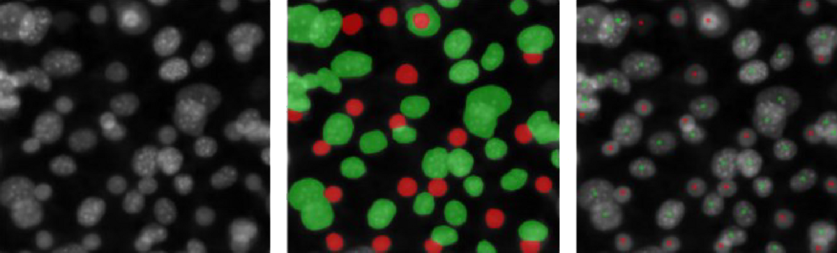
Fig 1: Original image, label for classic segmentation, label for dot-placing.
Preparing labels for classic segmentation requires much more effort than preparing labels for dot-placing, and the number of contiguous green regions does not simply correspond to the number of ‘green’ objects, in contrast to the number of green dots. Fluorescence microscopy images here and throughout from the dataset BBBC026v1. See below for attribution.
VAIDR is a system for automated microscopy, data management, and sophisticated, AI-based image analysis. It has recently been extended to support external image data in addition to data from the native VAIDR microscope. One of the features of VAIDR is a user-friendly user interface for labeling images for segmentation methods, training these methods, and applying them to new image data at scale. VAIDR also supports the user in the statistical analysis of the results generated by segmentation (and other) methods.
Results
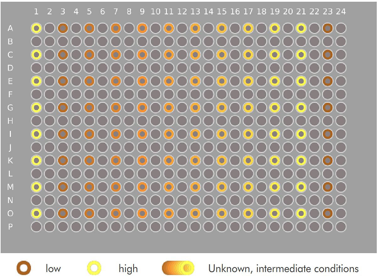
To illustrate the power of dot-placing for differential cell counting, and of the VAIDR system, we imported the publicly available cell image data set BBBC026v1.¹ This data set comprises images from 96 wells of a 384-well microtiter plate. The images are fluorescence images of the stained nuclei of a co-culture of (iPSC-derived) hepatocytes and murine fibroblasts. The hepatocyte seeding densities of the left-most and the right-most columns are given (‘low’ and ‘high’ condition, resp.); the culture conditions of the other wells are not supplied with the public dataset. The data set also comprises five images in which most nuclei are labeled as either those of a hepatocyte or a fibroblast by single red or green pixels respectively. Logan et al. 2015 present a CellProfiler pipeline implementing a cell counting method based on these data.
¹ Dataset BBBC026v1, by Anne Carpenter and David Logan, licensed under CC BY 3.0
We imported the image and meta data from that dataset into the VAIDR system. Then we iteratively
- reproduced one label from the original dataset using VAIDR’s point-and-click labeling UI,
- trained a new version of our counting method,
- evaluated all the data using the latest version of the method,
- corrected the placing of dots on the next labeled image from the original data set.
Accuracy
Naturally, when the task is to compare two methods for distinguishing things, accuracy is the go-to metric. However, in this case, the accuracy at predicting the labels from the original dataset is a bit problematic for several reasons:
- There are only five original labeled images. The statistics for prediction accuracy would therefore be weak in the best of cases, but also
- methodologically, we can only compare original labels with images that weren’t used to train our method. Since the last version of our model, which was trained on all labeled images, performs significantly better than the one before that (see below), all we can do is compare the performance of the known suboptimal version of our method on the one image it was not trained on. However, for lack of a better option, that is what we will do.
- Not all nuclei were labeled in the original images, and not all labeled nuclei are found by our method. Therefore, there are nuclei for which we cannot compare the classification by our method with the original labels. For the present analysis, we will only compare the classifications of nuclei that are both labeled and found by our method.
- Our method sometimes places a two-colored dot on a nucleus, generally indicating a difficult classification. There are multiple ways to deal with this, but for simplicity, we will count each dot that contains some red as a hepatocyte.
- Finally, the original labels were the subjective assessments of one or more researchers. Human assessments fluctuate and so we cannot expect them to be consistent. In fact, close inspection does seem to find the odd inconsistency. Since no method can learn random fluctuations, we should expect and in fact welcome differences between the results from our method and the original labels.
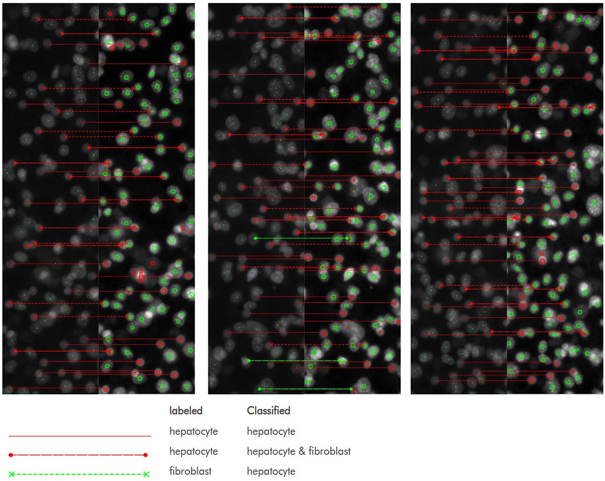
Fig 3 shows the original label and the result of the penultimate version of our method side by side. On this single image, the false-hepatocyte rate of this method is 0.085. While this can clearly be improved (and very probably is improved in the final version), it is clear that a red dot corresponds much more likely to a hepatocyte than to a fibroblast.
Separation of ‘High’ and ‘Low’ Condition
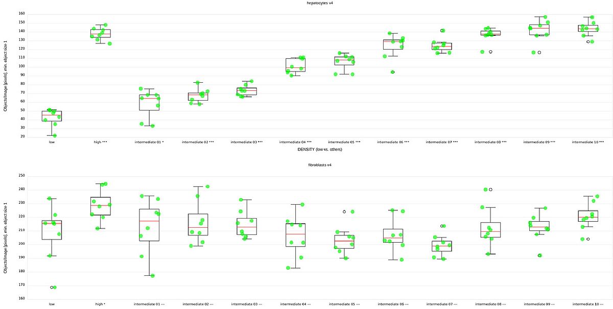
Logan et al. evaluated their pipeline mostly based on separation of the high and low condition. Fig 4, top and bottom show the median counts of hepatocytes and fibroblasts respectively, grouped by condition. We can see that the high and low condition are clearly separated in terms of hepatocyte count. We can also see the clear, systematic increase of hepatocyte counts across the unknown conditions, suggesting a serial dilution of something. However, as expected, no clear differences are visible between the numbers of fibroblasts.
| 2 | 3 | 4 | 5 | # Images in Training |
| -7.610 | 0.27 | 0.27 | 0.44 | z' |
Tab 1: Number of images in Training vs. z’ of separation between ‘high’ and ‘low’ condition.
Tab 1 shows the z’ values for the difference of the score distribution for the high and low conditions for each of the versions of our model. The populations are separated already after the first iteration (not shown), but the separation improves significantly even from the penultimate to the last step.
Clearly, with five labeled images, this method is more than adequate for counting hepatocytes in this setting.
At least as important as the somewhat qualitative performance analysis of our method above is the fact that developing it was a quick and easy exercise. It was a little more involved than usual because we had to make sure we were replicating the original labels exactly, but it was still much less work than finding the data, preparing the post-analysis, and writing this paper. We estimate that the time spent uploading the images into our system, labeling the images, and preparing the graphs took about six hours, plus breaks during which the machine worked and methods were trained.
Conclusion
Image-based differential cell counting is a good methodological fit for many research applications. To be practical and universally applicable, both imaging and image analysis must be cheap, fast and robust.
This leads to the need for a cost-efficient and streamlined workflow for method development and application as well as evaluation of quantitative results.
Using the example of dot-placing for differential cell counting, we demonstrated that the VAIDR system is an ideal platform for implementing such workflows.
References:
Logan DJ, Shan J, Bhatia SN, Carpenter AE (2015). Quantifying co-cultured cell phenotypes in high-throughput using pixel-based classification. Methods pii: S1046-2023(15)30170-5 / doi. PMID: 26687239. PMCID: PMC4766037.